User manual

RFscape is one page with three tools. This manual goes through them in the order you will use them: a link between two stations, the coverage of one repeater, the coverage of a network of repeaters. Every step says what to click and what to type, and every figure says what the page is telling you.

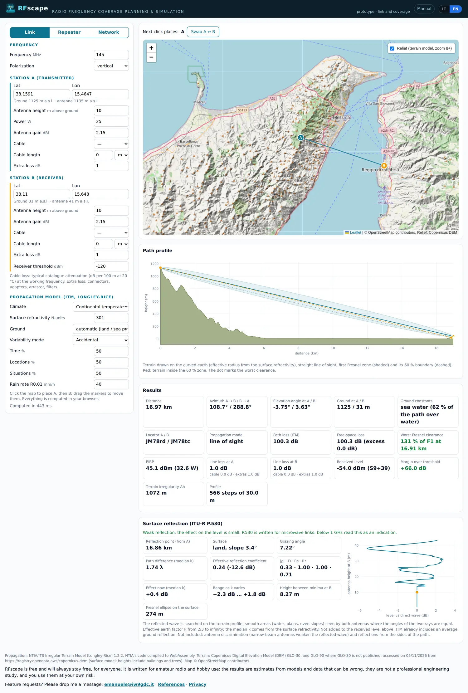
The screenshots show the page in English, its original language: the Italian version has the same layout, with the labels translated.

Quick start: a coverage map in five steps

If you only want to see something working before reading the details:

1. Open RFscape. The page starts in Link mode with an example link already computed across the Strait of Messina: marker A is on Monte Dinnammare and B is in Reggio Calabria.
2. Type the frequency. It is the first field, top left: 145 MHz for the 2 m band, for example.
3. Press Repeater. It is the middle of the three buttons above the parameters: the left panel becomes the repeater and the map a dashed circle around it.
4. Describe the station. Latitude and longitude of the site (or drag the marker), antenna height above ground, power in watts, antenna gain, cable and its length. Under the fields the page reads the ground from the terrain model and shows the antenna height above sea level: check it before going on.
5. Press Compute coverage. The button is under the map: in a few seconds the circle fills with colours, the legend at the bottom right gives the levels and the cards below the map summarise the area.

Everything is computed in your browser. Nothing is uploaded, there is no queue on a server, and the page works the same on a phone, only more slowly. The first computation of a new area also downloads its terrain, so it takes longer than the following ones.

The screen at a glance

All three modes share the same layout: parameters on the left, map on the right, answers below. What changes is which parameters you see and what the answers are.

• The mode buttons. Link, Repeater and Network, at the top left. Switching does not lose your work: each coverage mode keeps its own result and comes back ready.
• The parameters. Frequency and polarization first, then the stations, then the coverage (Repeater and Network) and the propagation model. The model block can stay as it is; see Common settings.
• The map. Click it to place a station or to read a point, drag the markers to move a site. The control at the top right switches the shaded relief on and off, from zoom 8 in.
• The answers. The path profile, the results and the reflection card in Link; the coverage summary in Repeater and Network, plus the repeater table in Network.

The setup is written in the address bar as you change it: to keep a job, copy the link. See Saving and sharing.

Part 1 - Link: can these two stations hear each other?

Link mode draws the terrain between two stations and answers two questions: is there a clear line of sight, and how much signal arrives at the receiver. It is the mode for a single contact, for a point-to-point link, and for understanding why a path that should work does not.

Step by step

1. Choose Link. The bar above the map says which station the next click will place, A or B.
2. Frequency and polarization. They are the first two fields. Polarization matters over water and on long paths; for FM voice, vertical is the usual choice.
3. Station A, the transmitter. Type Lat and Lon, or click the map and drag the marker. Under the coordinates the page writes the ground and the antenna height above sea level read from the terrain model, for example "Ground 1125 m a.s.l. - antenna 1135 m a.s.l.".
4. Power, gain, cable. Power is the transmitter output in watts. Height is above ground, not above sea level. Gain is the antenna gain in dBi. Choose the cable and its length in metres or feet: the line under the field gives the attenuation per 100 m, per 100 ft and over that run at the working frequency. Extra loss covers connectors, adapters, the lightning arrestor and filters.
5. Station B, the receiver. The same fields plus Receiver threshold, the level below which the receiver is silent. -120 dBm is an optimistic FM receiver, -110 dBm a realistic one, -100 dBm one in a poor site.
6. Read the profile. It is the drawing under the map: it shows whether the path is free and where the terrain comes closest to the line of sight.
7. Read the results. They are the cards below the profile.
8. Read the reflection card. It is at the bottom, for paths over water or flat land.

The link is recomputed a moment after every change, without pressing anything. If the numbers do not move, wait a fraction of a second and look at the status line at the bottom of the panel, which says "Computed in 40 ms" when it is done.

Reading the profile

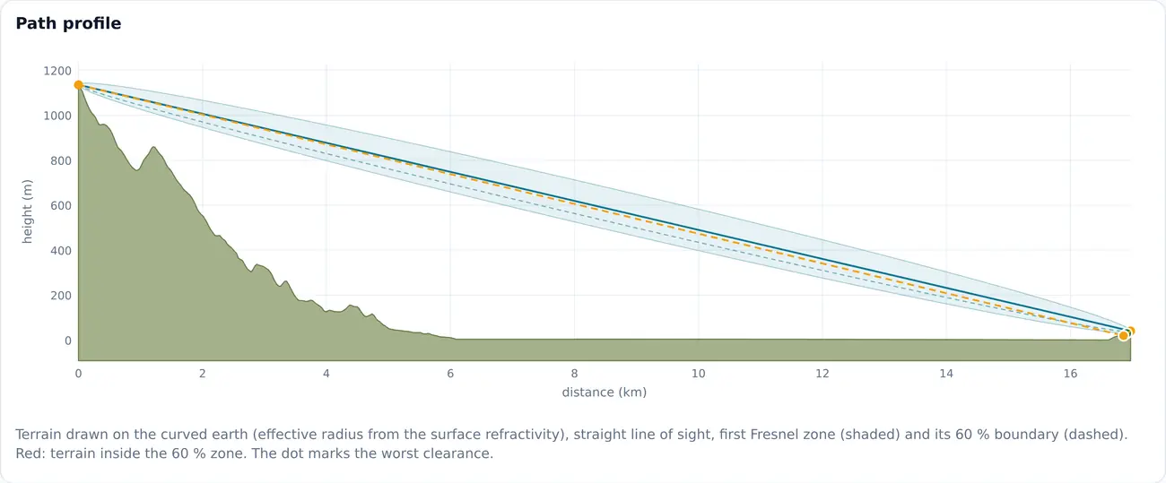
The terrain is drawn on the curved earth, with the effective earth radius taken from the surface refractivity: the two ends of the path bend downwards, so a link that looks straight on a flat drawing is not. The shaded band is the first Fresnel zone, the volume the radio waves need to be free; the dashed line is its 60 %, the usual working limit. Red segments are terrain inside that limit, and the dot marks the worst point of the path.

Move the mouse over the profile to read, point by point, the distance, the ground, the earth bulge, the height of the line of sight and the clearance as a fraction of the first Fresnel radius. The same point is marked on the map.

Reading the results

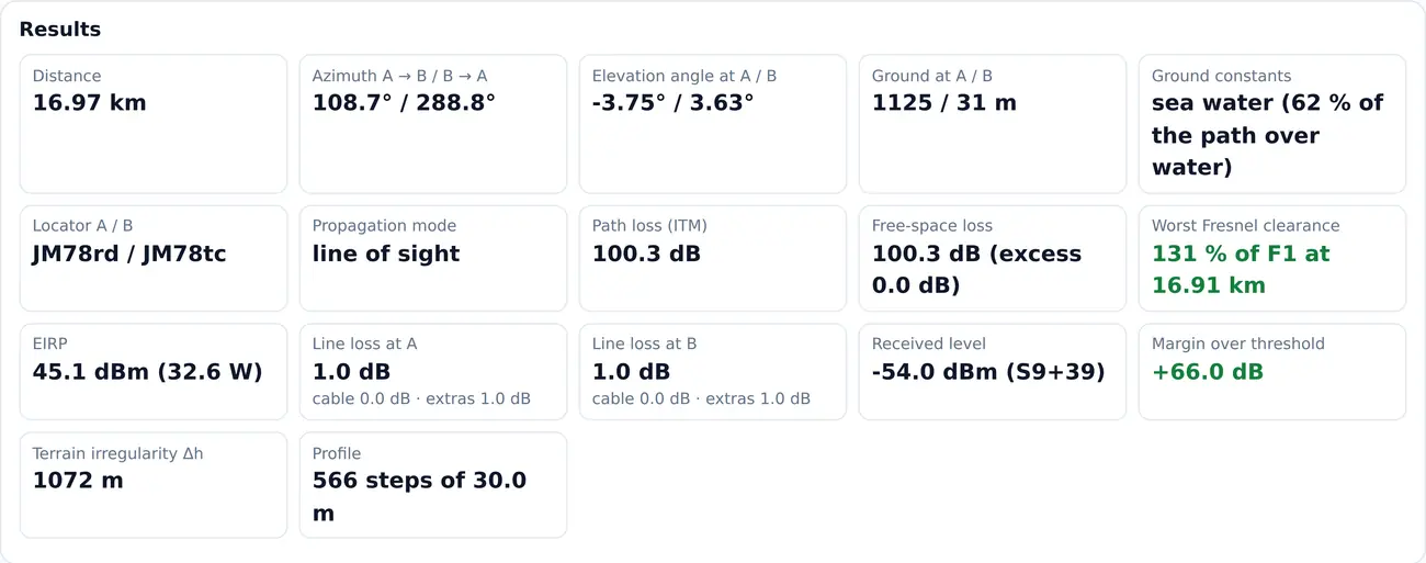
Distance, azimuth, elevation angles

The geometry of the path: how long it is, where B is seen from A and vice versa, and how much each antenna looks up towards the other. An elevation angle of a few degrees is normal on a long path over the earth's curvature.

Line of sight and worst Fresnel clearance

If the path is blocked, where and by how many metres; otherwise the worst clearance as a percentage of the first Fresnel radius. Above 60 % the path is clear, from 0 to 60 % it is partly obstructed, below zero it is blocked.

Path loss and free-space loss

The total loss predicted by the model, and what the same path would lose with nothing but air in the way. The excess, the difference between the two, is what the terrain costs.

EIRP

Power plus antenna gain minus line loss at the transmitter: what really leaves the antenna, in dBm and in watts.

Line loss at A and B

Cable and extras, split, so that a long run of thin coax does not hide in a single number.

Received level and margin over threshold

The level at the receiver terminals, with the S-meter equivalent, and how much it is above the threshold. Plus 10 dB or more is a comfortable link; 0 to plus 10 dB works, with fades; below zero the station is not heard.

Ground constants

What the model uses under the path. With automatic they are average land, with sea water where most of the path is water; the percentage says how much of the path is over water.

Propagation mode

The model's own classification of the path: line of sight, diffraction or tropospheric scatter. Diffraction is the normal mode beyond the radio horizon, and it falls quickly with distance.

Terrain irregularity and profile

How rough the terrain is, which the model uses to choose its curve, and how many steps the profile has (one every 30 m).

Gases and rain

From 1 GHz: the absorption of oxygen and water vapour, and the rain attenuation exceeded for 0.01 % of the year. The rain figure is an outage figure, not the everyday level: the card also shows the margin during that rain.

Surface reflections (ITU-R P.530)

Over water or flat ground part of the signal arrives at the receiver after bouncing off the surface, and adds to or subtracts from the direct wave. The card searches the profile for the point where the two paths have equal angles, then follows it as the effective earth radius changes with the weather.

• Reflection point, surface and grazing angle. Where the bounce is and on what: a reflection close to one antenna, or on rough ground, is weaker.
• Path difference, in wavelengths. Near 0, 1, 2 and so on the two waves add; near 0.5, 1.5 and so on they cancel.
• Minima crossed as k varies. How many times the level passes through a minimum when the atmosphere bends more or less. One or more minima with a strong reflection is the case to avoid, because it gives deep fades.
• Effective reflection coefficient. How much of the wave comes back, from 0 to 1; water is close to 1 at shallow angles.
• Effect now and range as k varies. The level change at the median atmosphere and the extremes it can reach.

The reflection is diagnostic: it is not added to the received level, because the propagation model already includes an average ground reflection. To fight it, change an antenna height until the reflection falls on rough or wooded ground, prefer vertical polarization over water, or use two antennas in space diversity, about half the height between minima apart.

Part 2 - Repeater: how far does one station reach?

Repeater mode answers the question of a repeater keeper: how far does my station reach, and what does a mobile hear at ground level along the way. It computes the level on every point of a circle around one station, for a mobile receiver on the ground.

Step by step

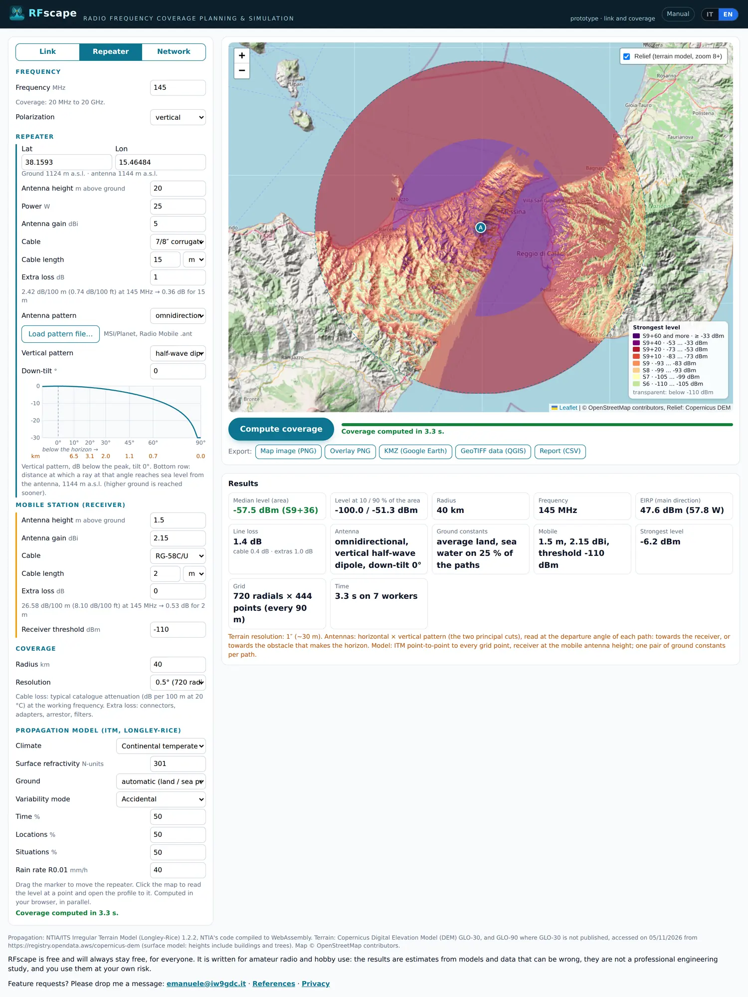
1. Choose Repeater. The map centres on the station with a dashed circle of the coverage radius.
2. Frequency and polarization. At the top, as in Link.
3. The site. Lat and Lon, or drag the marker. Watch the ground elevation shown under the fields: on a summit it is the number that decides the coverage.
4. Height, power, gain, cable, extra loss. As in Link. The height is the antenna's above the ground at the site, mast included.
5. Antenna pattern. Omnidirectional, directional (with azimuth, beamwidth and front-to-back ratio) or a pattern file. Load pattern file accepts MSI/Planet and Radio Mobile .ant files; the page fills in the gain and, if the file has it, the vertical pattern. The files stay in this browser.
6. Vertical pattern and down-tilt. The elevation diagram of the antenna, in dB below its peak. The small plot shows where a ray at each angle lands. A high gain collinear squeezes the signal towards the horizon: on a mountain a few degrees of down-tilt fill the valleys, but too much leaves a hole at the horizon.
7. Mobile station. Antenna height above ground (1.5 m for a car roof or a handheld), gain, cable, extra loss and threshold. Think twice about the threshold: every 6 dB is one more S-unit of coverage, and -120 dBm flatters any station.
8. Coverage. Radius and resolution, then press Compute coverage.

Radius and resolution

The radius is how far the computation goes, from 5 to 500 km. It does not change the colours, only where the map stops: keep it close to the distance you care about, because a smaller circle is computed sooner and read better.

The resolution is the angular step between radials: 360 radials (1°) is a quick preview, 720 (0.5°) the normal choice, 1440 (0.25°) for maps that go into a report. One-degree radials make spokes on sharp ridges, where the map reads a crest along one ray and a valley along the next: if the result looks striped, raise the resolution.

Reading the map

• Colour is the received level at the mobile. The legend at the bottom right gives each colour in dBm and in S-units: S9 is -93 dBm above 30 MHz, 6 dB per S-unit, and the scale stops at S9+60.
• Transparent is below the threshold. There the mobile does not hear the repeater.
• The dashed circle. It is the radius you asked for, not the limit of the coverage.
• Click a point. A popup gives the levels at that point and a button opens the profile from the repeater to it. This is the quickest way to understand why a valley is dark.

The summary below the map

Median level over the computed area, the levels at 10 % and 90 % of it (the pessimistic and the optimistic end), radius, frequency, EIRP, the antenna as it was described to the model, the mobile, the grid actually computed and the time it took. The median is the number to compare when you change a height or a power: 6 dB more is one S-unit everywhere.

The five exports

Map image (PNG)	The map as it is on screen: background, coverage, repeaters, legend and credits. For a message or a slide.
Overlay PNG	Only the coverage layer, transparent outside it, with its bounds in the note. To lay it over another map or a drawing.
KMZ (Google Earth)	Coverage, legend and repeaters for Google Earth.
GeoTIFF data (QGIS)	Not a picture: four bands with the strongest level in dBm, the best server, the number of repeaters received and the field strength in dBµV/m, georeferenced in WGS 84. For QGIS, ArcGIS or a script.
Report (CSV)	Model parameters and data sources, then the level every 5 km on radials every 30°, with field strength and margin. The format regulators and filings ask for.

The exports use the last computed coverage. If the bar under the map is amber, press Compute coverage first or the file will contain the old map.

Part 3 - Network: which repeater serves which area?

Network mode puts several repeaters on one map and answers the question that matters when a network is planned: which repeater serves each area, and where two of them are heard at once. It is the same engine as Repeater, run for every repeater and then combined point by point.

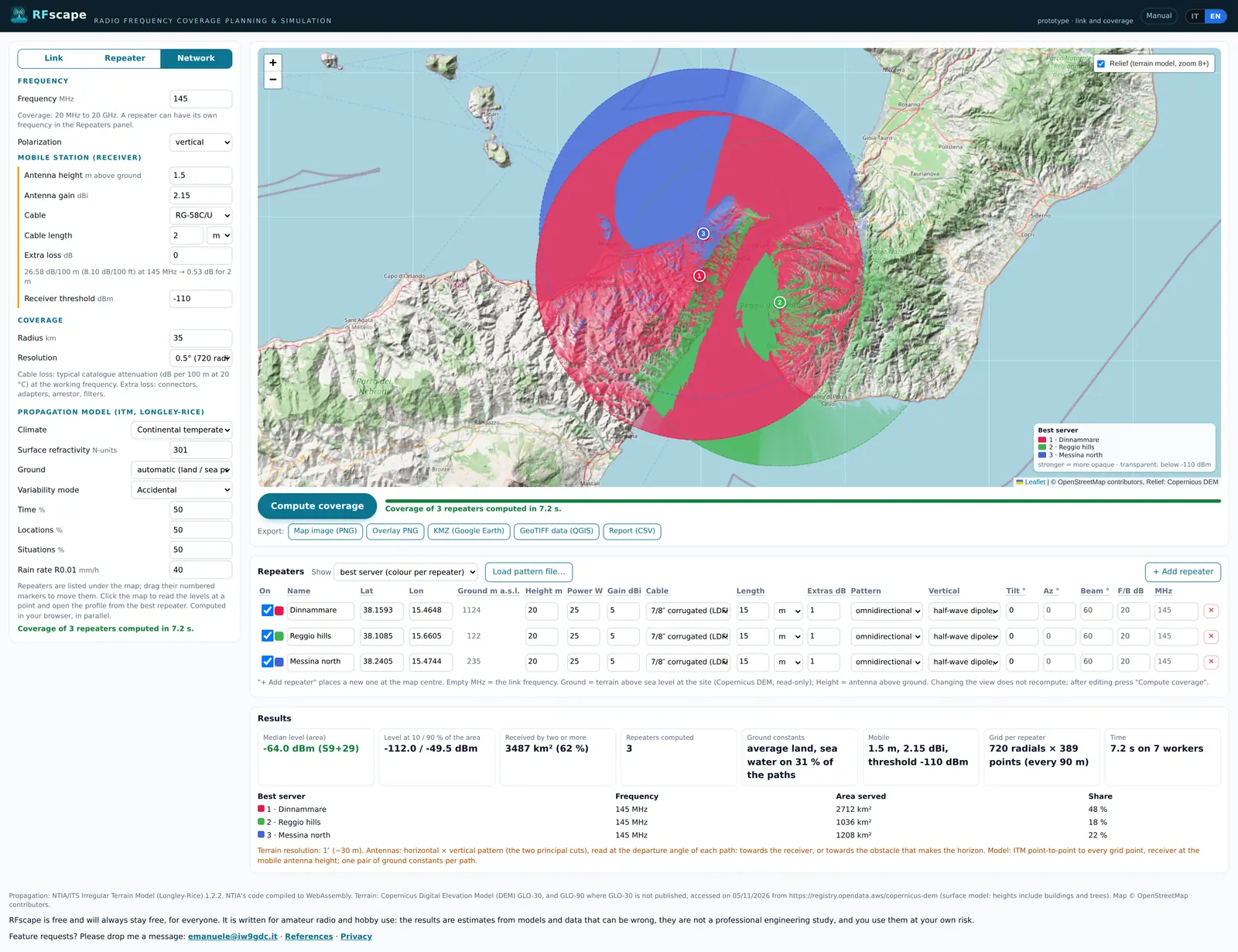
Step by step

1. Choose Network. The map changes to the repeaters and their numbered markers.
2. Fill the table. One row per repeater: + Add repeater places a new one at the centre of the map with the parameters of the last one. Change the coordinates (or drag the marker) and, if it is a different station, power, gain, antenna and cable. An empty MHz means "the frequency at the top"; a repeater on another band can have its own.
3. Ground m a.s.l. This column is read from the terrain model and cannot be edited: it is there to keep a site choice honest. Height is the antenna above that ground.
4. On. This checkbox switches a repeater in or out of the computation without deleting it: use it to compare two candidate sites.
5. Press Compute coverage. The button is under the map; the bar and the message say when it is done, and the time grows with the number of repeaters, the radius and the resolution.
6. Choose the view. Use Show, then read the results.
7. Iterate. Move a marker, change a height or a power, press Compute coverage again and look at what changed.

The three views

Best server (colour per repeater)

One colour per repeater, drawn where that repeater gives the strongest level. It is the map of the network: who serves what. The colour is more opaque where the signal is stronger, and transparent where no repeater reaches the threshold.

Strongest level (S-units)

The S-meter scale of the strongest repeater at each point, without saying which one it is. It shows the general gradient: where the network is strong, where it is thin.

Overlaps (repeaters received)

How many repeaters are above the threshold at each point. One is normal service, two or more is an overlap: a receiver with tone squelch has a choice, a receiver without one may hear both.

Changing the view does not recompute: the levels are the same and only their combination changes. That is the point of the mode: compute once, read the network in three ways.

Reading the results

Median level over the whole network area with the 10 % and 90 % ends, the area reached by two or more repeaters, the number of repeaters computed, the ground constants, the mobile, the grid per repeater and the time. Below them, one row per repeater with the area it serves best and its share: the quickest way to spot a repeater that is doing nothing, or one that carries the network alone.

How to plan with it

• Start from your real sites and your real antennas, not from ideal ones: the map is only as good as the table.
• Look for the dark areas inside the circle and click them: the profile from the best repeater usually says whether the problem is distance or a ridge.
• If two repeaters overlap almost perfectly, one of them is in the wrong place: switch one off and see what the other covers alone.
• A hole between two areas is often better filled by moving a site a few hundred metres than by doubling the power.
• Before believing a coverage, change the receiver threshold by 6 dB and compute again: if the edge moves a lot, the result depends on a number you do not know exactly.

The settings common to all modes

The block at the bottom of the left panel is the propagation model. The defaults are right for most work in Italy, and these are the fields worth knowing.

Frequency

From 20 MHz to 20 GHz. Above 1 GHz the page adds the absorption of gases and the rain figure.

Polarization

Vertical or horizontal. It changes the ground reflection and, above 1 GHz, the rain attenuation.

Climate

Seven climate types of the Longley-Rice model: continental temperate inland, maritime temperate over land along the coasts, maritime temperate over sea for a path that is mostly water. It moves the curve in diffraction and scatter, not on a clear line of sight.

Surface refractivity

How much the atmosphere bends the radio waves, in N-units. 301 is the temperate median and 250 to 400 covers the usual range: a lower value bends less, so the radio horizon is nearer.

Ground

Automatic is a good default: average land, sea water where most of a path is over water. The other choices force one pair of constants (poor, average, good, fresh water, sea water). Forcing sea water everywhere makes an inland map optimistic.

Variability mode

How the model treats the variations: single message, accidental, mobile or broadcast. Accidental is the usual for a fixed link, mobile for a station that moves.

Time, locations, situations

The percentages of time, places and situations in which the predicted level is exceeded. 50 % is the median; lower percentages give a more conservative level, because they are exceeded less often.

Rain rate R0.01

The rain intensity exceeded for 0.01 % of the year, in mm/h, used from 1 GHz. 40 mm/h is a reasonable value for Italy; the maps of ITU-R P.837 give the local figure.

Receiver threshold

The level below which the receiver is silent. It is not a property of the model: it decides where the colours stop, and it should be the threshold of the real receiver, not the best one on the market.

The cable list uses typical catalogue values, in dB per 100 m at 20 °C and at the working frequency. Makers' figures differ by a few per cent between batches: read them as plus or minus 10 %.

Saving and sharing your work

The whole setup is written in the address bar as you change it: coordinates, heights, powers, cable, model and repeaters. Copy the link and you have saved the job: opening it again gives the same page, ready to compute. It is also the easiest way to ask for help, because it shows exactly what you had on screen.

Two things do not travel in the link: the antenna pattern files, which stay in the browser where they were loaded (the page asks for them again elsewhere), and the computed coverage, which is never stored: a link opens the setup, then the computation runs again.

Exports are files, not projects: the KMZ, the GeoTIFF and the CSV are made to be opened elsewhere. Saved projects, with a name and a list, are what the free account is for; until then, keep the links.

When something does not work

Ground: no terrain data here

The point is outside the terrain published for the page. Move the station or check the coordinates: a swapped latitude and longitude is the usual cause, Italy being around 38°N and 15°E.

TILE: ... (4 attempts ...)

A terrain tile did not arrive. Press Compute coverage again: the second attempt usually finds it in the cache. On a slow connection, a smaller radius helps.

Parameters changed: press "Compute coverage"

The map on screen was computed with the previous values. Nothing is lost: press the button.

Spokes or stripes in the coverage

One-degree radials on a sharp ridge. Compute at 0.5° or 0.25°.

The computation takes a long time

It runs in parallel in your browser, on as many workers as the cores minus one. Radius, resolution and the number of repeaters are the cost: start with 30 km at 0.5°, then widen.

Everything is pink, or everything is dark

Check the threshold first, because -120 dBm makes almost everything audible, then the antenna gain and the cable: 50 m of thin coax instead of 5 m eats the whole budget. Then check the frequency: 145 with 1300 in mind gives quite another map.

The map image is not available

A background tile arrived without permission to be copied into the image. Reload the page and press the button again.

The results are estimates from models and data that can be wrong, and the terrain model contains buildings and trees: treat them as a planning aid, not as a measurement.